
NIOS Class 12 Economics Chapter 23 Revenue And Profit Maximization of a Competitive Firm, Solutions to each chapter is provided in the list so that you can easily browse through different chapters NIOS Class 12 Economics Chapter 23 Revenue And Profit Maximization of a Competitive Firm and select need one. NIOS Class 12 Economics Chapter 23 Revenue And Profit Maximization of a Competitive Firm Question Answers Download PDF. NIOS Study Material of Class 12 Economics Notes Paper 318.
NIOS Class 12 Economics Chapter 23 Revenue And Profit Maximization of a Competitive Firm


Also, you can read the NIOS book online in these sections Solutions by Expert Teachers as per National Institute of Open Schooling (NIOS) Book guidelines. These solutions are part of NIOS All Subject Solutions. Here we have given NIOS Class 12 Economics Chapter 23 Revenue And Profit Maximization of a Competitive Firm, NIOS Senior Secondary Course Economics Solutions for All Chapters, You can practice these here.
Revenue And Profit Maximization of a Competitive Firm
Chapter: 23
Module – VIII: Market And Price Determination
TEXT BOOK QUESTIONS WITH ANSWERS
INTEXT QUESTIONS 23.1.
Q.1. Define TR, AR and MR symbolically.
Ans. (i) Total Revenue: The money income received by a firm by selling units of production in the market is known as total revenue i.e., if we multiply the goods sold with the price it will give total revenue.
TR = Quantity Sold x Price
(ii) Average Revenue: Total revenue when divided total number of units sold given average revenue.
AR = TR/ Quantity sold
Average revenue is always equal to the price of the commodity. This can be
(iii) Marginal Revenue: The addition in the total revenue with the sale of an addition unit of the product i.e., MR = TRₙ – TRₙ–₁.
or MR = ΔTR / ΔQuantity sold
Q.2. If price is 5 and quantity sold increases from 6 to 7, find out TR, AR and MR. Where P = Price, Q = Quantity and Δ = increase in.
Ans.
| P | Q₁ | TR | AR | MR |
| 5 | 6 | 30 | 5 | 5 |
| 5 | 7 | 35 | 5 | 5 |
INTEXT QUESTIONS 23.2.
Q.1. The average cost of a firm is 10. It sold 10 units at a price of 10. What type of profit did the firm coin?
Ans. The firm can earn the normal profit and zero profit.
Q.2. If TR > TC, then there is normal profit. (True or False)
Ans. True.
Q.3. If TR = TC, thin there is super normal profit. (True or False)
Ans. False.
Q.4. If AR > AC, then there is loss. (Ture or False)
Ans. False.
INTEXT QUESTIONS 23.3.
Q.1. Maximum profit implies that MC is above MR after both are equal. (True or false)
Ans. True.
Q.2. At quantity 2, TR = TC. After that TC lies below TR and again they become equal at quantity. 6. Do you firm agree that profit maximizing output lies between these two quantities. (Yes/ No)
Ans. Yes.
TERMINAL EXERCISE
Q.1. Define total revenue, average revenue and marginal revenue. Give their relationship.
Ans. Total revenue refers to total receipts from the sale of a given quantity of a commodity. It is the total income of a firm. Total revenue is obtained by multiplying the quantity of the commodity sold with the price of the commodity.
Total Revenue = Quantity x Price
For example, if a firm sells 10 chairs at a price of ₹ 160 per chair, then the total revenue will be 10 Chairs x ₹ 160 = ₹ 1,600.
Average Revenue (AR): Average revenue refers to revenue per unit of output sold. It is obtained by dividing the total revenue by the number of units sold.
Average Revenue = Total Revenue/Quantity
For example, if total revenue from the sale of 10 chairs @ ₹ 160 per chair is ₹ 1,600, then:
Average Revenue = Total Revenue/Quantity = 1,600/10 = 160.
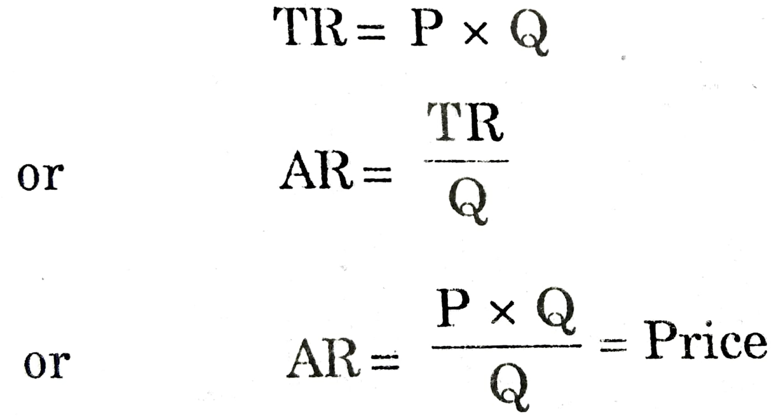
AR and Price are the Same: We know, AR is equal to per unit sale receipts and price is always per unit. Since sellers receive revenue according to price, price and AR are one and the same thing.
This can be explained as under:
TR = Quantity x Price …….. (1)
AR = TR/ Quantity …………. (2)
Putting the value of TR from equation (1) in equation (2), we get
AR = Quantity x Price/ Quantity
AR = Price
AR Curve and Demand Curve are the Same: A buyer’s demand curve graphically represents the quantities demanded by a buyer at various prices. In other words, it shows the various levels of average revenue at which different quantities of the good are sold by the seller. Therefore, in economics, it is customary to refer AR curve as the Demand Curve of a firm.
Marginal Revenue (MR): Marginal revenue is the additional revenue generated from the sale of an additional unit of output. It is the change in TR from sale of one more unit of a commodity.
MRₙ = TRₙ – TRₙ_₁
Where:
MRₙ = Marginal revenue of nth unit.
TRₙ = Total revenue from n units.
TRₙ_₁ = Total revenue from (n-1) units; n = number of units sold. For example, if the total revenue realised front sale of 10 chairs is ₹ 1,600 and that from sale of 11 chairs is ₹ 1,780, then MR of the 11th chair will be:
MR₁₁ = TR₁₁ – TR₁₁
MR₁₁ = ₹1,780 – ₹1,600
= ₹180
One More way to Calculate MR: We know, MR is the change in TR when one more unit is sold. However, when change in units sold is more than one, then MR can also be calculated as:
MR = Change in Total Revenue/ Change in number of units
= ∆TR/∆Q
Let us understand this with the help of an example: If the total revenue realised from sale of 10 chairs is 1,600 and that from sale of 14 chairs is 2,200, then the marginal revenue will be:
MR = TR of 14 chairs – TR of 10 chairs/
= 14 chairs – 10 chairs
= 600/ 4
= ₹ 150
TR is summation of MR: Total Revenue can also be calculated as the sum of marginal revenues of all the units sold.
It means, TRₙ = MR₁ + M₂ + MR₃ +……….MRₙ
or TR = ∆MR.
Q.2. Fill TR, AR and MR column.
| P | Q | TR | AR | MR |
| 20 | 4 | |||
| 20 | 5 | |||
| 20 | 6 |
Ans.
| P | Q | TR | AR | MR |
| 20 | 4 | 800 | 20 | 20 |
| 20 | 5 | 100 | 20 | 20 |
| 20 | 6 | 120 | 20 | 20 |
Q.3. Distinguish between super normal nad normal profit.
Ans. The surplus income received by deducting total costs from total revenue is called profits. These profits may be of two types-normal profits and super normal profits.
Normal profit: Normal profit is the opportunity cost of the entrepreneur which he must receive i.e., normal profits are the profits which are necessary for the entrepreneur so as to continue in the industry i.e., if even normal profits are not received in the long run, the firm has no reason to continue in the long run. This, is the amount which other firm in the industry are receiving. These profits are received by the entrepreneur of bearing risk or for management, etc. Normal profits as such is the part of the average cost and it affects the price of the product. When average revenue of a firm is equal to its minimum average cost, the firm is said to be earning normal profits. Under the conditions of perfect competition and even monopolistic competition firms earn normal profits in the long run.
Supernormal profit (abnormal profit): These profits are a type of surplus received by the entrepreneur or a type of surplus rent received by him in the short run due to the scarcity of factors of production, however, ‘such profits vanish in the long run. Such profits do not enter into costs. When average revenue is more than the average costs, the firm is earning supernormal profits. Difference between AR and AC denotes profits per unit and when multiplies by the total units sold it gives the total supernormal profits. In the case of monopoly a firm is in a position to earn super normal profits in the short run as well as in the long run.
Q.4. Write a short note on loss of a firm by giving numerical example.
Ans. An operating loss indicates that a company’s core operations are not profitable and that changes need to be made either to increase revenues or to decrease costs. An operating loss is sometimes expected for certain start-up companies which incur high costs in an attempt to grow quickly.
In most other situations, an operating loss is a sign of potential distress at a company. An operating loss can be a particularly dire indicator for a company heavily financed with debt because the company has lost money even before considering interest payments, which may be substantial.
Q.5. Explain profit maximisation principle by using TR and TC approach. Give suitable example.
Ans. There are two approaches to explain the equilibrium or profit maximisation by the firm:
(a) Total-revenue and total cost approach, and
(b) MR and MC approach.
Though in modern economic analysis, the equilibrium of a firm is usually explained through MR & MC approach, for some purposes total revenue and total cost approach is highly useful (for example, to show breakeven level of output).
Therefore, we first explain how a perfectly competitive firm maximises its economic profits using total revenue and total cost curves. Since under perfect competition marginal revenue is constant, total revenue curve is an upward-sloping straight line. On the other hand, due to varying returns to the factors used, Total Cost (TC) curve first increases at a decreasing rate and then after a point it increases at an increasing rate.
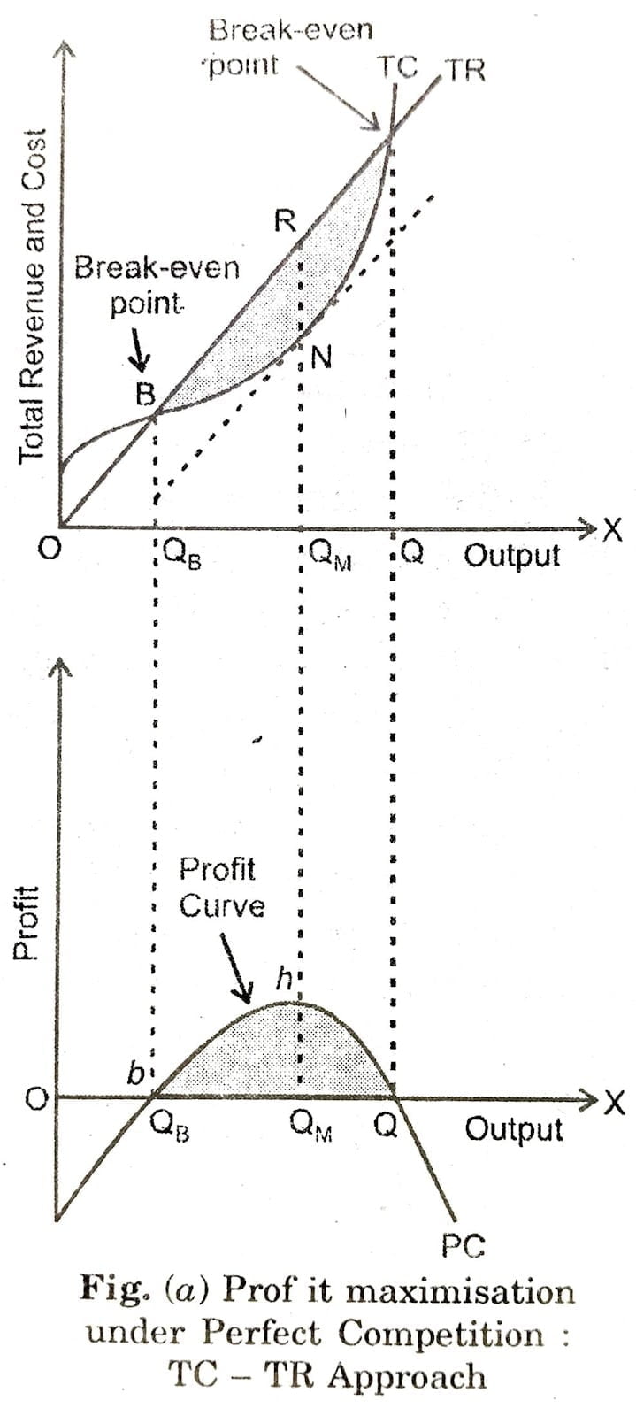
Equilibrium of a firm working under perfect competition which aims at profit maximisation is graphically illustrated in Figure (a) where TR represents total revenue curve and TC represents total cost curve. Total revenue curve starts from the origin which means that when no output is produced, total revenue is zero.
As output is increased total revenue goes on increasing at a constant rate. This is because price for a firm working under perfect competition remains constant whatever its level of output. Consequently, total revenue curve TR is a straight line from the origin.
However, it will be noticed that the.total cost curve TC starts from a point F which lies above the origin. It means that OF is the fixed cost which the firm has to incur even if it stops production in the short run. It will be seen that the short-run total cost curve TC initially increases at a decreasing rate and then after a point it increases at an increasing rate.
This implies that average total cost curve is roughly of U-shape. Total profits can be measured as the vertical distance between the TR and TC curves. It will be observed from Fig. (a) that upto the level of output OQB TC curve lies above TR curve showing that as the firm raises its output in the initial stages total cost is greater than total revenue and the firm is incurring losses.
When the firm produces OQB level of output, total revenue just equals total cost and the firm is therefore neither making profits, nor losses. That is, the firm is only breaking even at output level OQB. Thus, the point B or output level OQB is called Break-Even Point.
When the firm increases its output beyond OQB total revenue becomes larger than total cost and therefore profits begin to accrue to the firm. It will be noticed from the Fig. (a) that profits are increasing as the firm increases production to output OQM, since the distance between the total revenue curve (TR) and Total Cost Curve (TC) is widening. At OQM level of output, the distance between the TR curve and TC curve is the greatest and therefore profits will be maximum.
If the firm expands output beyond QM, the gap between TR and TC curves goes on narrowing down and therefore the total profits will be declining. It is therefore clear that the firm will be in equilibrium at QM level of output where total revenue exceeds total cost by the largest amount and hence its profit. maximum. It will be observed from Figure (a) that at output level QU, total revenue is again equal to total cost (TR curve cuts TC curve at point K corresponding to output QU). Thus, point K is again a breakeven point, usually called upper breakeven point.
It may however be noted that this upper break-even point K or output level QU is not of much relevance as it lies beyond firm’s profit maximising level and may actually lie beyond firm’s capacity to produce. It is the first break-even point B or output level QB which is highly significant as a firm will not plan to produce if it cannot sell output equal to at least QB at which total revenue just covers total cost of production so that its economic profits are zero.
For a more vivid representation of profit maximising level of output we have drawn in the low panel of Figure (a) the profit curve PC which measure the distance between TR and TC curves. It will be see from this lower panel of Fig. (a) that up to output level QB profit curve lies below the X-axis showing that the firm is making losses if it produces less than QB.
At output level QB the firm’s economic profits zero because at this output level total revenue just cover total cost of production. Therefore, output QB is break even level of output. As the firm expands its level output beyond QB, profit curve is rising until it reach its maximum point corresponding to level of output Q.
Beyond level of output QM, profit curve slope downward indicating that profits decline beyond output QM. Thus, at output level QM, the firm maximise economic profits. At a higher output level profits a gain zero indicating the upper break-even point.
There is a major shortcoming of the TC and TR approach of analysing firm’s equilibrium. It is that this approach what price will be charged by the firm its equilibrium position is not directly mown. Therefore in what follows we explain the modern MC = MR approach to firm’s equilibrium.
Q.6. Explain profit maximisation conditions a competitive firm by using suitable diagram.
Ans. Perfect competition arises when there many firms selling a homogeneous good to many buyers with perfect information.
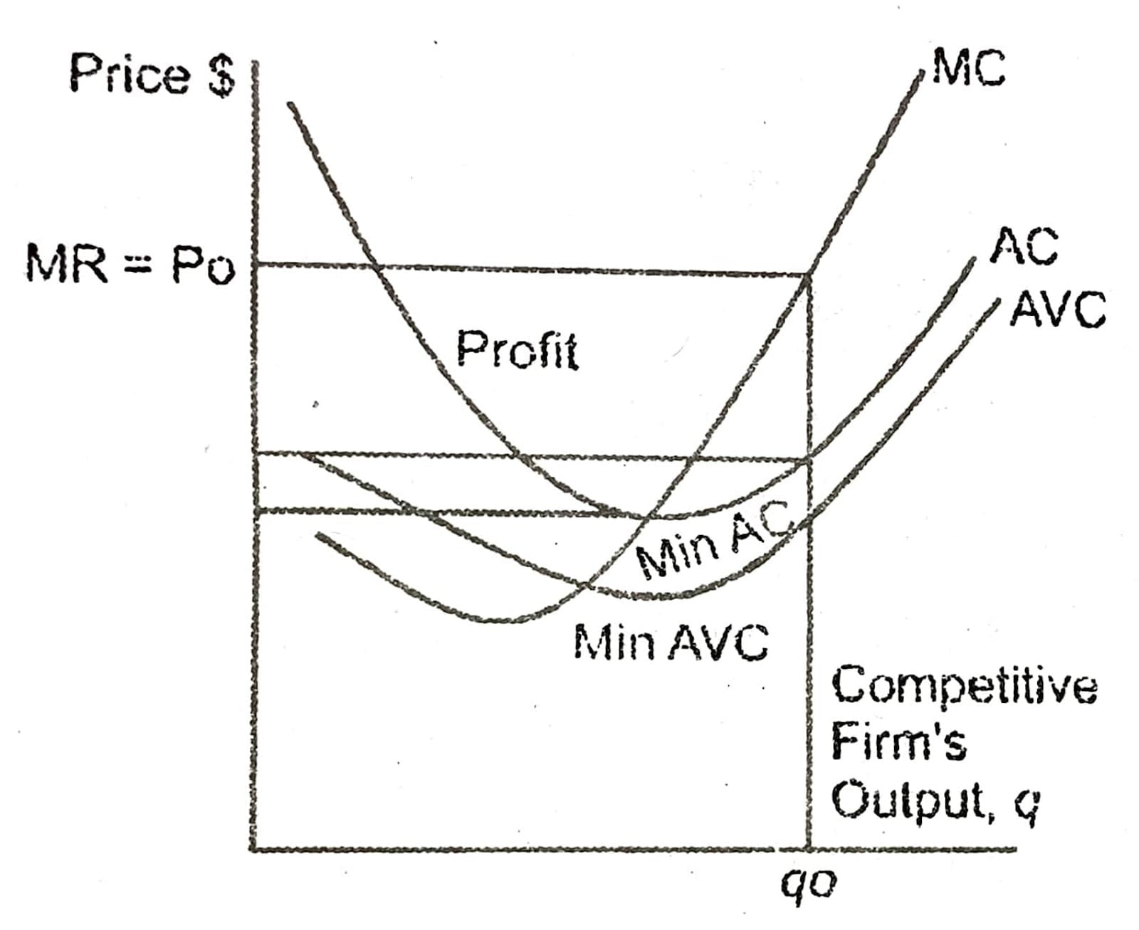
Under perfect competition firm is a price taker of its good since none of the firm can individually influence the price of the good to purchased or sold. As the objective of each perfect competitive firm, they choose each of their output levels to maximize their profits. The key goal for a per competitive firm in maximizing its profits is to calculate the optimal level of output at which its Marginal Cost (MC) = Market Price (P). As shown in the graph the profit maximization point is where MC intersect with MR or P. If the above competitive firm produces quantity exceeding Qo, then MR and Po would be less than MC, the firm would incur an economic loss on the marginal unit, so the firm could increase its profits decreasing its output until it reaches go. If the above competitive firm produces a quantity fewer than qo, the MR and Po would be greater than MC, the firm would incur profit, but not to its maximum. Therefore, the firm could increase its profits by increasing its output untill reaches qo.
Q.7. Construct an imaginary table show the profit maximisation output by using TR and TC approach.
Ans. A firm attains the stage of equilibrium when it maximises its profits, i.e. when he maximises the difference between TR and TC. After reaching such a position, there will be no incentive for the producer to increase or decrease the output and the producer will be said to be at equilibrium.
According to TR-TC approach, producer’s equilibrium refers to stage of that output level at which the difference between TR and TC is positively maximized and total profits fall as more units of output are produced. So, two essential conditions for producer’s equilibrium are:
The difference between TR and TC is positively maximized.
Total profits fall after that level of output.
The first condition is an essential condition.
But, it must be supplemented with the second condition. So, both the conditions are necessary to attain the producer’s equilibrium.
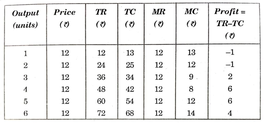
Producer’s Equilibrium (When Price remains Constant): When price remains same at all output levels (like in case of perfect competition), each producer aims to produce that level of output at which he can earn maximum profits, i.e. when difference between TR and TC is the maximum. Let us understand this with the help of Table below, where market price is fixed at ₹ 10 per unit:
According to Table, the maximum profit of 9 can be achieved by producing either 3 units or 4 units. But, the producer will be at equilibrium at 4 units of output because at this level, both the conditions of producer’s equilibrium are satisfied:
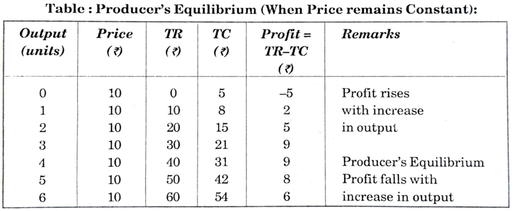
1. Producer is earning maximum profit of 9.
2. Total profit falls to 8 after 4 units of output.
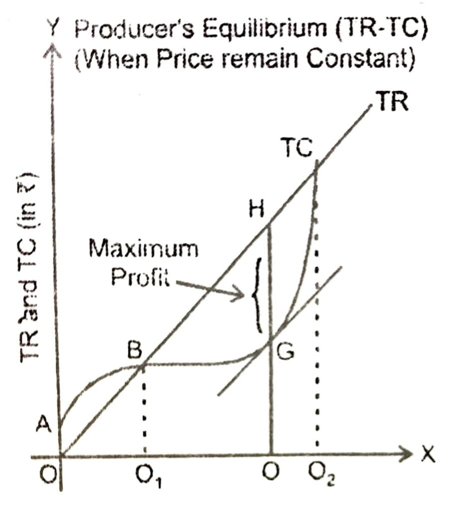
In Fig. below, Producer’s equilibrium will be determined at P OQ level of output at which the vertical distance between TR and TC curves is the greatest. At this level of output, tangent to TC curve (at point G) is parallel to TR curve and difference between both the curves (represented by distance GH) is maximum.
At quantities smaller or larger than OQ, such as OQ₁ or OQ₂ units, the tangent to TC curve would not be parallel to the TR curve. So, the producer is at equilibrium at OQ units of output.
Producer’s Equilibrium (When Price Falls with rise in output): When price falls with rise in output (like in case of imperfect competition), each producer aims to produce that level of output at which he can earn maximum profits, i.e. when difference between TR and TC is the maximum. Let us understand this with the help of Table ahead:
According to Table, MC = MR condition is satisfied at both the output levels of 2 units and 5 units. But the second condition, ‘MC becomes greater than MR’ is satisfied only at 5 units of output. Therefore, Producer’s Equilibrium will be achieved at 5 units of output. Let us now discuss determination of equilibrium with the help of a diagram:
Producer’s Equilibrium is determined at OQ level of output corresponding to point K as at this point:
(i) MC = MR; and
(ii) MC is greater than MR after MC = MR output level.
Output is shown on the X-axis and revenue and costs on the Y-axis. Both AR and MR curves are straight line parallel to the X-axis. MC curve is U-shaped. Producer’s equilibrium will be determined at OQ level of output corresponding to point K because only at point K, the following two conditions are met:
1. MC = MR; and
2. MC is greater than MR after MC = MR output level.
Although MC = MR is also satisfied at point R, but it is not the point of equilibrium as it satisfies only the first condition (i.e., MC = MR). So, the producer will be at equilibrium at point K when both the conditions are satisfied.
Some Other Important Questions For Examinations
Very Short Answer Type Questions
Q.1. Define revenue.
Ans. Revenue is the money receipts from the sale of the product.
Q.2. Define total revenue.
Ans. Total revenue is the total amount of money received by the firm from the sales.
Q.3. Define average revenue.
Ans. Average revenue is the price per unit revenue received from the sale of one unit of a commodity.
Q.4. How can average revenue be obtained?
Ans. It can be obtained by dividing totál revenue by the quantity sold.
Q.5. Define marginal revenue.
Ans. Marginal revenue is the addition to total revenue by the sale of an additional unit of the commodity.
Q.6. Is average revenue equal to the price?
Ans. Yes, average revenue is equal to the price.
Since, AR = P × Q/ Q
Hence, AR = P.
Q.7. What is the shape of total revenue curve facing a competitive firm?
Ans. The total revenue curve facing a competitive firm is a straight line parallel to X-axis.
Q.8. When will total revenue start declining?
Ans. Total revenue starts declining when marginal revenue is less than zero, i.e. negative.
Q.9. What is the slope of total revenue curve facing a competitive firm?
Ans. The total revenue curve facing a competitive firm is a straight line passing through the origin.
Q.10. What is the shape of A.R. and MR curves?
Ans. AR and MR curves are horizontally straight lines in case of perfect competition whereas, they are downward sloping curves under imperfect competition.
Q.11. What is the break even point?
Ans. The break even point refers to a situation where total cost and total revenue are equal. At this point the firm gets only normal profit.
Q.12. What is the shape of AR curve under monopoly and monopolistic competition?
Ans. AR curve has a steep slope under monopoly but the firm under monopolistic competition faces an elastic average revenue curve.
Q.13. What is shut-down point?
Ans. Shut-down point refers to a situation where average revenue is equal to average variable cost. If the price falls to cover even average variable cost, firm will stop its production.
Q.14. How are the marginal revenue and the average revenue curves under monopoly and imperfect competition?
Ans. Under monopoly and imperfect competition, marginal revenue and average revenue curves are not only separate from each other but are also downward sloping.
Q.15. In monopolistic competition, marginal revenue is less than average revenue. Give reasons.
Ans. A monopoly firm has to reduce its price to sell more output in the market.
Q.16. Under which market condition MR will be zero?
Ans. In monopoly or monopolistic condition MR will be zero.
Q.17. When average revenue is constant, what is the state of marginal revenue?
Ans. When average revenue is constant, marginal revenue is also constant and equal to average revenue.
Q.18. What is the shape of marginal revenue curve and average revenue curve under perfect competition?
Ans. Under perfect competition both marginal revenue and average revenue curves are represented by one curve which is parallel to OX-axis.

Hi! my Name is Parimal Roy. I have completed my Bachelor’s degree in Philosophy (B.A.) from Silapathar General College. Currently, I am working as an HR Manager at Dev Library. It is a website that provides study materials for students from Class 3 to 12, including SCERT and NCERT notes. It also offers resources for BA, B.Com, B.Sc, and Computer Science, along with postgraduate notes. Besides study materials, the website has novels, eBooks, health and finance articles, biographies, quotes, and more.