
Class 11 Economics Chapter 4 The Theory of The Firm under Perfect Competition, (Assam Higher Secondary Education Council) AHSEC Class 11 Economics Question Answer in English Medium each chapter is provided in the list of AHSEC so that you can easily browse through different chapters and select needs one. Assam Board Chapter 4 The Theory of The Firm under Perfect Competition Class 11 Economics Question Answer can be of great value to excel in the examination.


AHSEC Class 11 Economics Chapter 4 The Theory of The Firm under Perfect Competition
Class 11 Economics Chapter 4 The Theory of The Firm under Perfect Competition Notes cover all the exercise questions in SCERT Textbooks. The SCERT Class 11 Economics Chapter 4 The Theory of The Firm under Perfect Competition Solutions provided here ensure a smooth and easy understanding of all the concepts. Understand the concepts behind every chapter and score well in the board exams.
The Theory of The Firm under Perfect Competition
LONG ANSWER QUESTIONS TYPE : (MARKS : 5)
1. What is price elasticity of supply ? How can it be measured? Explain.
Ans : Price elasticity of supply is the measure of change in supply of a commodity due to change in its price. According to Samuelson, “Elasticity of supply is the degree of responsiveness of supply of a commodity to a change in its price.” And according to Prof. Bilas, “Elasticity of supply is defined as the percentage change in quantity supplied, divided percentage change in price.” The price elasticity of supply, denoted by is defined as follows―
Price elasticity of supply(es) = Percentage change in quantity supplied/ Percentage change in price.
Price elasticity of supply is measured by dividing proportionate change in supply by proportionate change in price.
Es = Proportionate change in supplied
Proportionate change in price.

Q=initial Quantity, Q₁ = New Quantity, P₁ = New price, P= initial price, ΔQ=Change in Quantity, Δ P = Change in price.

2. Explain different kinds of price elasticities of supply by using the geometric method.
Ans : There are five types of elasticity.of supply.
They are:
(i) Perfectly elastic supply : Perfectly elastic supply results in an infinite change in quantity due to a very small change in price.
In the figure, SS is perfectly elastic Supply curve. It is parallel to ox axis. implies that a slight fall in price will ace the supply to zero.

(b) Perfectly inelastic supply : Perfectly inelastic supply states that there is no change in supply, regardless of change in price. In the fig. SS is perfectly inelastic supply curve and is parallel to Y axis. It signifies that even if price increases to OP₁, the supply remains unchanged i.e., OS. In this case, elasticity of zero. Supply of perishable goods in short period is inelastic.

(c) Unitary elastic supply : If the resulting proportionate change in supply equals the given proportionate change in price, then elasticity of supply equals unity. In the fig. SS is the unitary elastic supply curve. This is clear from the fact that an increase in price from OP₁ to OP, is attended by a proportionate change in supply from OS to OS₁.

(d) More than unitary elastic supply : In this case, proportionate apply More than unitary elastic supply : In this case, proportionate is than proportionate change in price. In the fig. SS curve expresses more than unity elasticity of supply. When price increases, supply extends more than proportionately.
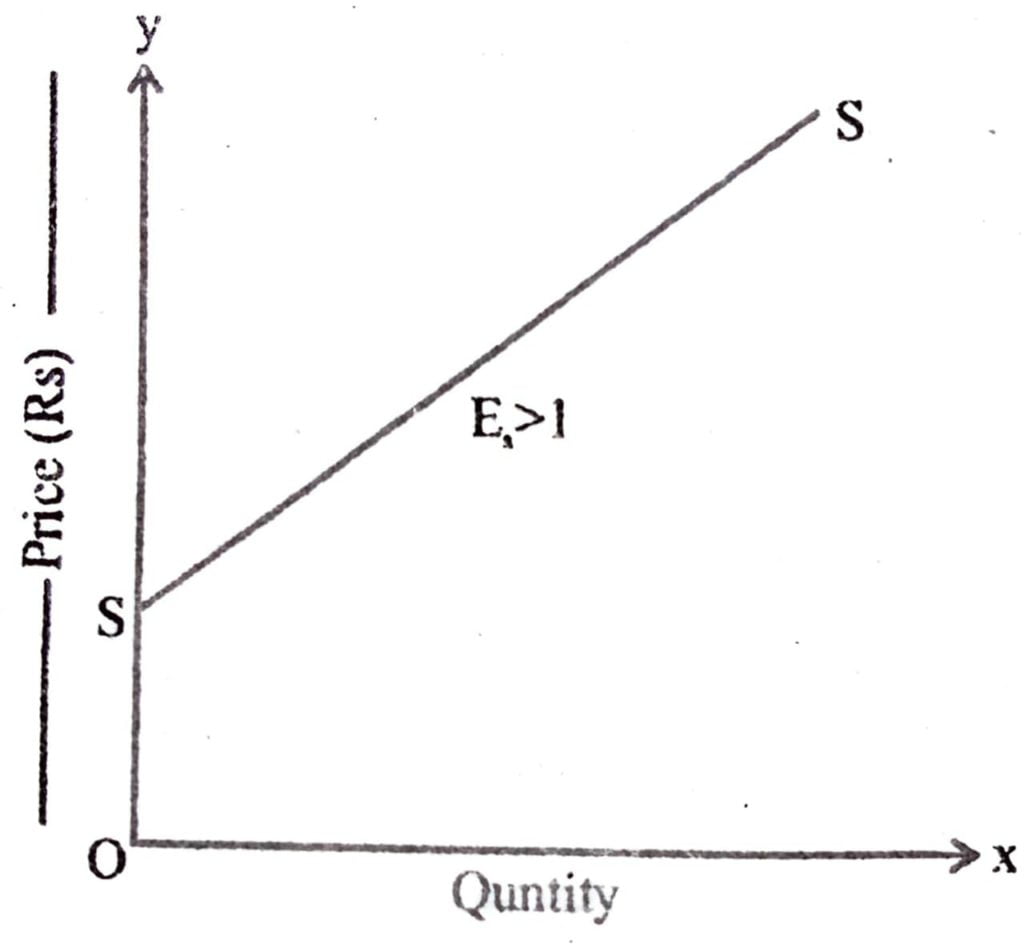
(e) Less than unitary elasticity : In this case, the proportionate change in quantity supplied is smaller than the proportionate change in price.
In the fig. supply curve SS represents less than unitary elasticity. When price increases, then supply extends less than proportionately.

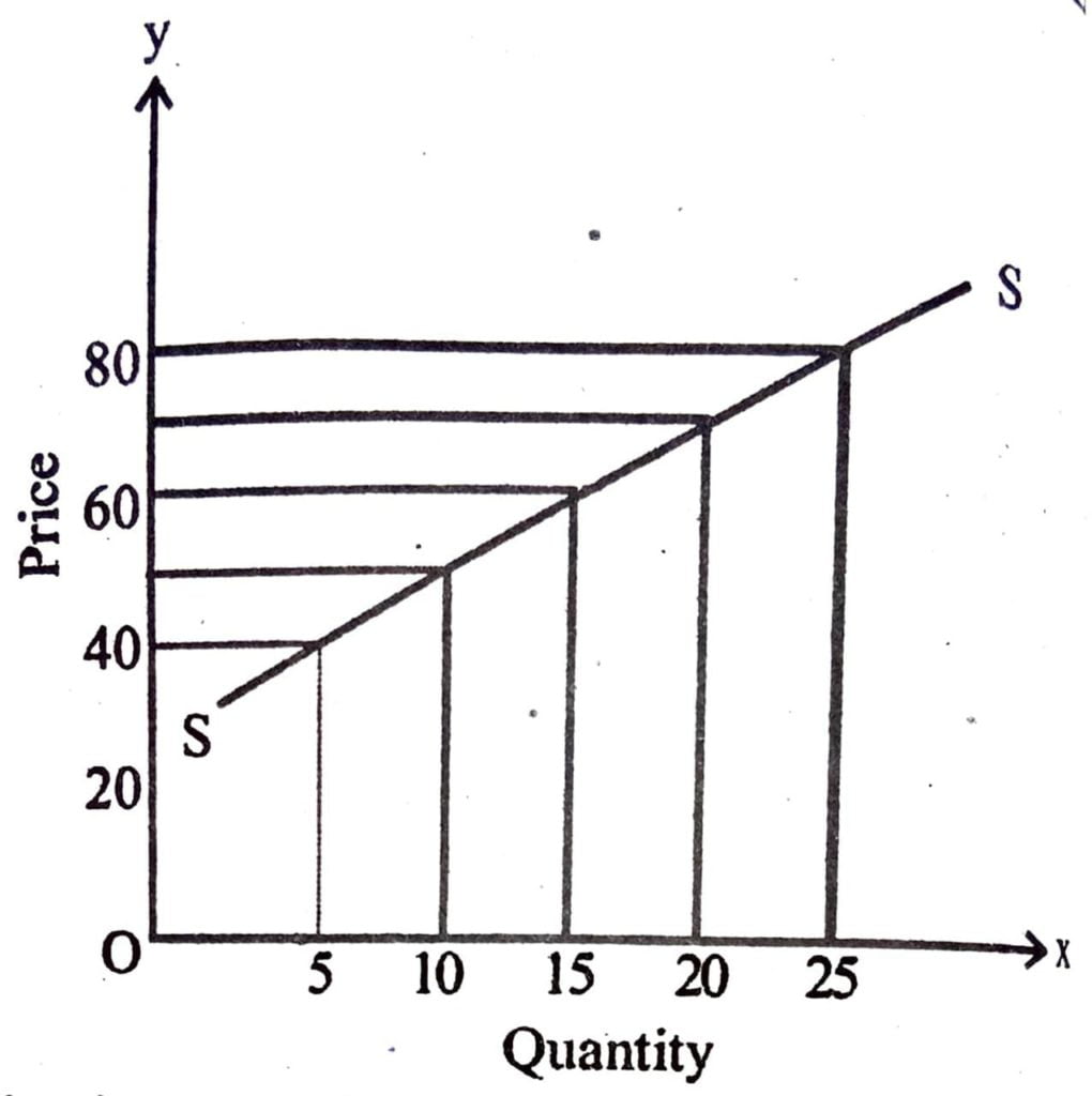
3. Explain how is the market supply curve derived.
Ans : The market supply curve shows the output levels that firms in the market produce in aggregate, corresponding to different values of the market prices. The supply curve slopes upwards from left to right showing that price and quantity supplied move in the same direction. A supply curve can be a straight line or a curve. The things that are kept constant in defining supply schedule and in drawing a supply curve are, the technology in the production of the commodity, the supplies of inputs, climate and weather conditions, wages, interest, prices of machinery, prices of raw materials etc.
Market supply schedule for commodity X.

There are, of course, y exceptions to the law of supply. It is most possible that in the case of some commodities, supply may not change in response to a change . in price. In the fig. SS is the market supply curve. In the ox axis, quantity supplied is measured and in the vertical oy axis, price per quintal is measured. As the price is increased, quantity supplied is also increa sed.
4. What is the shut-down point for the firms under perfect competition. Explain it with the help of a diagram.
Ans : Break even point 4. occurs when for a firm TR=TC (Total Revenue Total Cost)
In the long run, a firms must achieve this point. Shut down occurs when for. a firm
TR=TVC (Total Revenue= Total variable cost) In the short run, a firm must achieve this point.

5. Derive long-run supply curve of a firm under perfect competition and explain.
Ans:

The long run supply curve can be derived by two ways. Firstly. determine the firms’s profit maximising output level, when the market price is greater than or equal to the minimum AC. In the diagram, when market price is P₁ it exceeds the minimum LRAC. Upon equating P₁ with LRMC on the rising part of the LRMC curve, we obtain output level q₁. But LRAC at q₁ does not exceed the market price P₁. Thus, when market price is P, the firm’s supplies in the long run become an output equal to q₁.
After the first way is done, we determine the firm’s profit maximising output level, when the market price is less than the minimum of long run AC. If a profit maximising firm produces a positive output in the long , the market price P₂ must be greater than or equal to LRMC at the output level. But we have seen in the earlier diagram that for all positive output level, LRAC strictly exceeds P₂, In other words, it cannot be the case that the firm supplies a positive output. So, when the market price is P₂ the firm produces zero output.
By the two ways, we derive that a firm’s long run supply curve is the rising part of the LRMC curve from and above the minimum LRAC, pro pro together with zero output for all prices less than the minimum LRAC as shown in the diagram beside.
6. Graphically represent how a firm minimises its profits after satisfying the three conditions needed for it.
Ans : For any positive level of output, the following three conditions neet to be satisfied for a profit-maximising firm in the short run.
(i) P= SMC (Short run marginal cost)
(ii) SMC is non-decreasing
(iii) P> AVC LRMC

In the short run, the firm will not produce any level of output where market price is less than AVC. The firm can bear losses only up to the extent of total fixed cost, as fixed costs have to be borne when output is zero. In other words, total revenue at least must be equal to or greater than the TVC. Price should at Jeast be equal to AVC. It is only then the total loss borne by the firm will be maximum equal to TFC.
7. Explain why a profit maximising firm under competitive market will not produce at an output level where in the market price is lower than the AC in the long run.
Ans : A profit-maximising firm in a competitive market will not produce a positive level of output in the long run, if the market price is less than the minimum of AC. It is shown with the help of a diagram.
In the diagram, at output level q₁, the market price P is lower than the long run AC (LRAC) and q₁ can not be profit-maximising output level because firm’s total revenue TR at q, is the area of the rectangle OPAq₁, is while the firm’s total cost TC is the area of the rectangle OEBq₁. Since the area OEBq₁, is larger than the area of rectangle OPAq₁, the firm incur a loss at the output level q,. But in the long run setup a firm that shut down he production has a profit of zero. This means of course, that q₁ is not a C, profit-maximising output level.
A profit-maximising firm in a competitive market will produce a positive level of output in the long run when price must be greater than or equal to ter AC.
8. Suppose the price of a product under perfectly competitive market is Rs. 10. Calculation the total revenue (TR), marginal revenue (MR) and average revenue (AR) in the following table.hu

Ans:

9. The total cost (TC) and total revenue (TR) schedule of a firm under perfectly competitive market is given in the table. On the basis of that find out―

(a) the price of the product. (1)
(b) the profit schedule corresponding to each level of output
Ans:

10. ‘Under perfect competition in the long-run price must be greater than or equal to AC’- Explain with suitable example.
Ans: See Q. No. 7, (Long Type).
11. Let there be four firms in a perfectly competitive market. All these firms have similar supply curve (SS). Calculate the market.
Ans: See Q. No. 7, (Short Type I).
12. Under perfectly competitive market, the total cost (TC) function of a firm is given below. If the price of the commodity is Rs. 15, how much quantity of the commodity the firm would produce? What will be the total fixed cost ?
Ans: See Q. No. 8,(Short type I).
13. “In perfect competition, AR-MR but in monopoly AR>MR.” _Explain.
Ans: Under perfect competition market, neither the individual firm nor an individual consumer has any control over the price of the product. Thus, they will have to adjust with the prevailing market price. At the prevailing market price, an individual firm can sell as much as it likes. As single price prevails in the market, thus, for an individual firm, there is no difference between its average revenue (AR) and marginal revenue (MR), SO AR= MR.
A mathematical connection between average revenue and marginal
revenue stating that the change in the average revenue depends on a comparison between average revenue and marginal revenue. For perfect competition, with no market control, marginal revenue is equal to average
revenue, and average revenue does not change. For monopoly and other firms with market control, marginal revenue is less than average revenue, and average revenue falls.
The relation between average revenue and marginal revenue’, 500,400)”> marginal revenue is one of several that reflect the general relation between a marginal and the corresponding average. The general relation is this:
If the marginal is less than the average, then the average declines.
If the marginal is greater than the average, then the average rises. If the marginal is equal to the average, then the average does not change.
This general relation surfaces throughout the study of economics. It also applies to average and marginal product, average and marginal cost, aver age and marginal factor cost, average and marginal propensity to consume, and well, any other average and marginal encountered in economics.
14. The demand and supply function of a firm under perfectly competitive market are given below :
D=25-5P
S=-5+10P
where, D⇒ quantity demanded, S⇒ quantity supplied and P⇒ price. Find the equilibrium price, quantity demanded and quantity supplied.
Ans: D = 25-5P
S= -5+10P
D=S
⇒25 – 5P = – 5+10P ⇒ -5P – 10P = – 5 – 25 ⇒ -15P – 30 ⇒ P = 2
∴ P= 2
Equilibrium Price (P) = 2
D = 25-5P = 25-5×2 = 25-10 =15
S = -5+10 P = -5+ 10 × 2 = -5+20 =15
15. The total cost (TC) and prices (P) at different units of output of a monopolist are given below :
(i) Find out the total revenue (TR), marginal revenue (MR) and marginal cost (MC) schedules.
Ans:


Hi, I’m Dev Kirtonia, Founder & CEO of Dev Library. A website that provides all SCERT, NCERT 3 to 12, and BA, B.com, B.Sc, and Computer Science with Post Graduate Notes & Suggestions, Novel, eBooks, Biography, Quotes, Study Materials, and more.
