
Class 11 Economics Chapter 3 Production & Costs, (Assam Higher Secondary Education Council) AHSEC Class 11 Economics Question Answer in English Medium each chapter is provided in the list of AHSEC so that you can easily browse through different chapters and select needs one. Assam Board Chapter 3 Production & Costs Class 11 Economics Question Answer can be of great value to excel in the examination.
AHSEC Class 11 Economics Chapter 3 Production & Costs


Class 11 Economics Chapter 3 Production & Costs Notes cover all the exercise questions in SCERT Textbooks. The SCERT Class 11 Economics Chapter 3 Production & Costs Solutions provided here ensure a smooth and easy understanding of all the concepts. Understand the concepts behind every chapter and score well in the board exams.
Class 11 Economics Chapter 3 Production & Costs
SHORT ANSWER QUESTIONS TYPE-I: (MARKS : 4)
1. Draw the total product curve typical firm and explain it.
Ans:
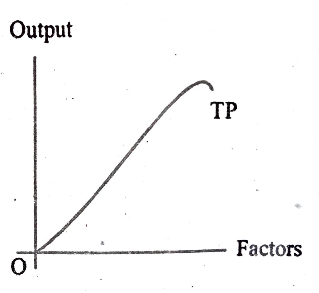
In figure above, TP is the typical total product curve of a firm which changes as the amount of factors increase/decrease.
2. Define long-run average cost and long-run marginal cost and explain their nature wit the help of corresponding curves.
Ans : For the first unit of output, both long run marginal cost and the average cost are the same. Then as output increases, long run average cost (LRAC) initially falls, and than after a certain point, it rises. As long.
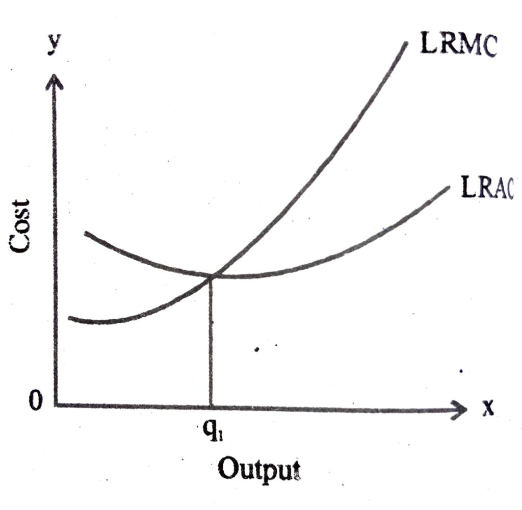
as average cost is falling, marginal cost is rising, marginal cost must be less than the average cost. When average cost is rising, marginal cost must be greater than the average cost. LRMC curve is therefore a ‘U’ shaped curve. It cuts the LRAC curve from below at the minimum point of the LRAC. In the diagram, long run marginal cost and the average cost curves drawn.
3. Explain the relationship between average product and marginal product with the help of diagram.
Ans: The diagram follows
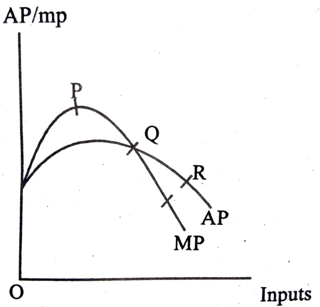
The relationships are :
(i) When MP> AP, AP rises, part P in the diagram.
(ii) When MP= AP, AP is maximum, point Q in the diagram.
(iii) When MP<Ap, AP falls, part R in the diagram.
4. Show that the average fixed cost curve is a rectangular hyperbola.
Ans: Average fixed cost equals to total fixed cost divided by output.The average fixed cost curve is downward sloping from left to right. It is shown in the diagram beside.
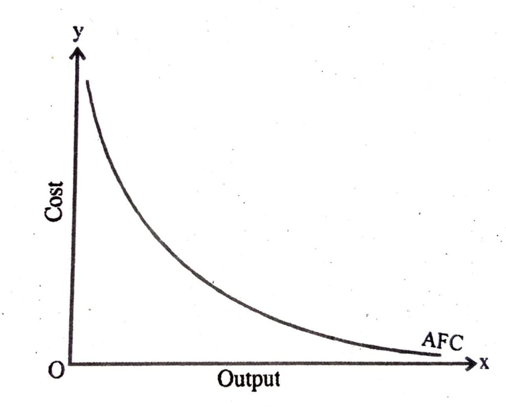
AFC is the average fixed cost curve, which is sloping downward to right. It look so due to its very nature, as the production goes on increasing. average fixed cost goes on diminishing.
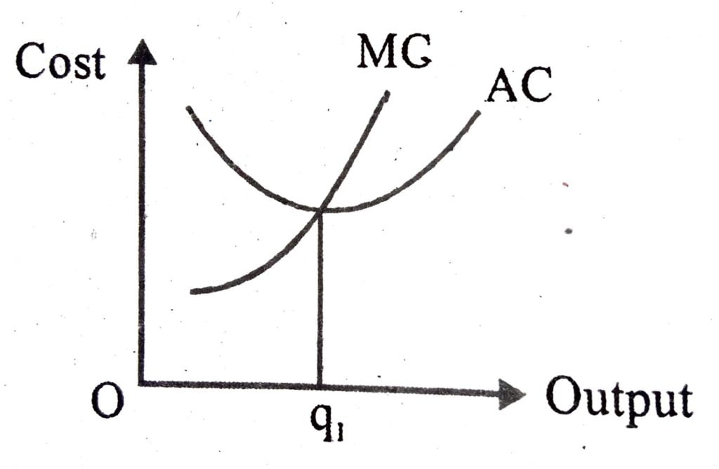
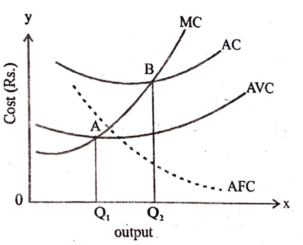
5. Draw and explain the shape of the average variable cost curve.
Ans: The shapes of short run marginal cost (SMC), average variable cost (AVC) and short run average cost (SAC) curves are shown in the diagram beside-
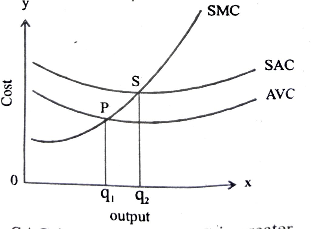
AVC reaches its minimum at q₁ units of output. To the left of q₁, AVC is falling and SMC is less than AVC. To the sight of q₁, AVC is rising and SMC is greater than AVC. SMC curve cuts the AVC curve at ‘P’, SAC which is the minimum point of AVC curve. The minimum point of SAC 8 is ‘S’, which corresponds to the output q, It is the intersection point between SMC and SAC curve. To S. AVC the left of q₂, SAC IS fall and SMC ndino greater is less than SAC, To the right of q₂, SAC is rising and SMC is SI 9 than SAC.
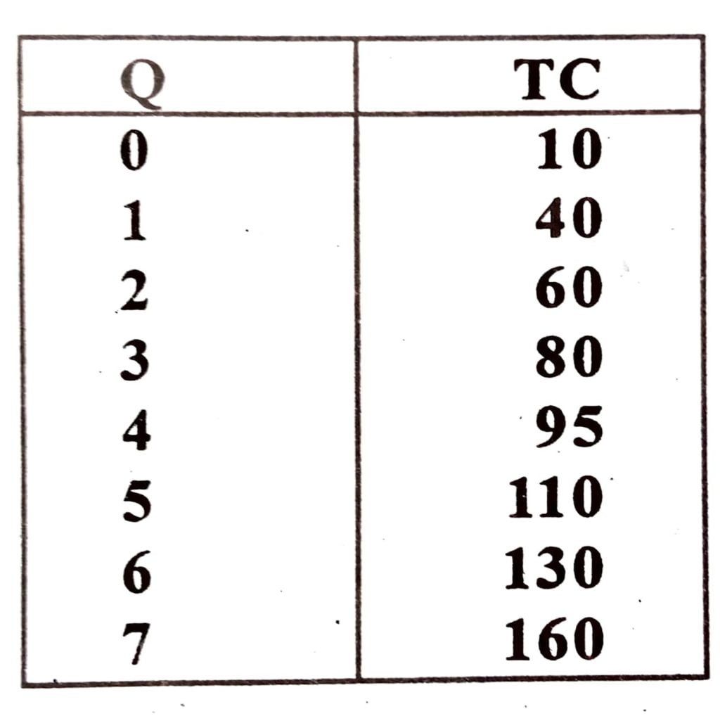
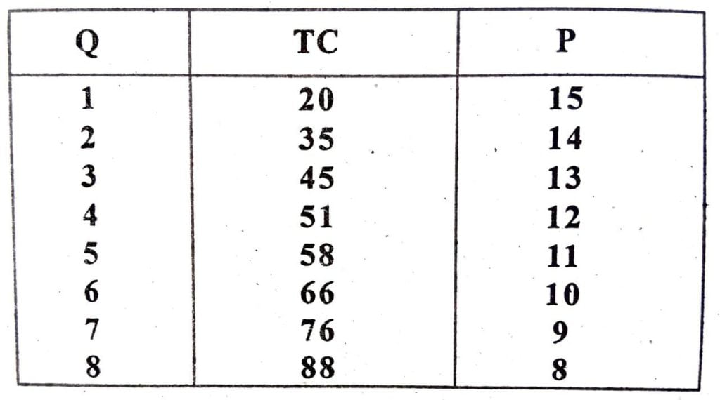
6. The total cost (TC) schedule of a production unit is give below. Find out the average cost (AC) schedule for the production unit.
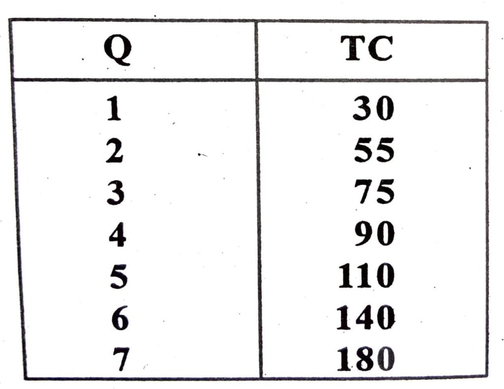
Ans:
7. The production function of a firm is given as :
Q=5L¹/₂ K¹/₂ Calculate the level of output when it employs 25 units of labour (L) and 9 units of capital (K).
Solution: Given Q=5L¹/₂K₁/₂
When L=25 units and K = 9 Units
∴ Q = 5(25)¹/₂(9)¹/₂ = 5×5×3
∴ Q=75 units
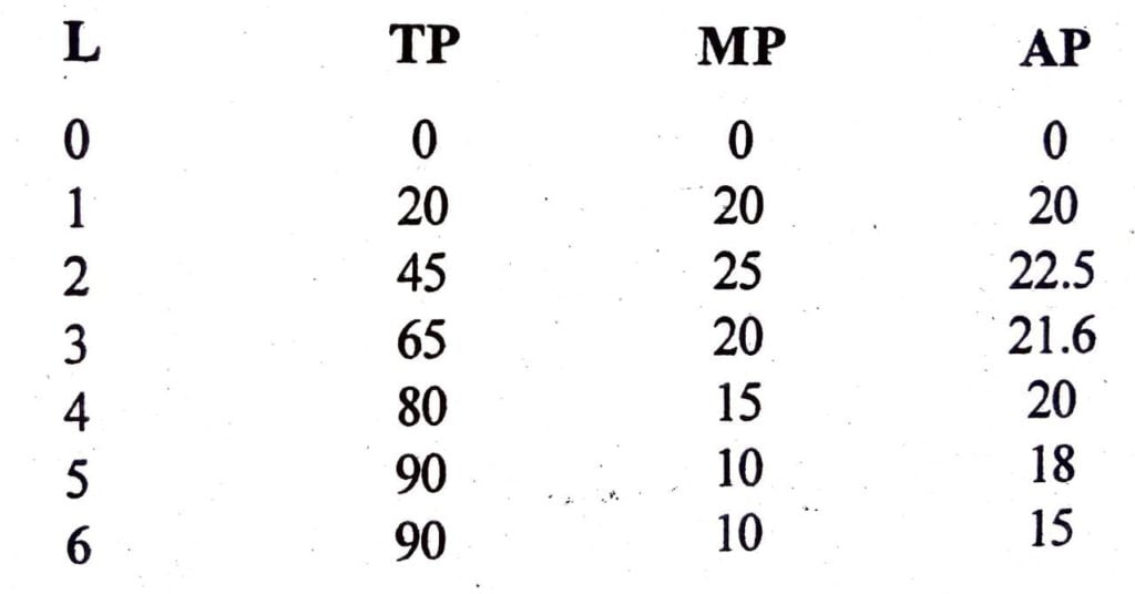
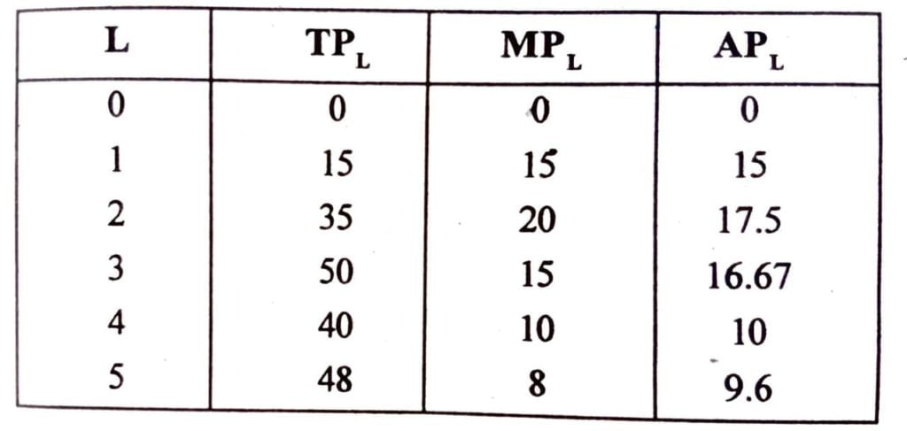
8. The total product schedule of a firm is given below:
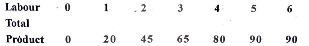
Calculate the marginal product and average product of the firm.
Ans:
9. Show the relationship between Average cost and marginal cost with a diagram.
Ans:
The relationship is:
(i) when average costs (AC) falls with an increase in output, MC always remains lower than AC.
(ii) when AC is rising, marginal cost (MC) remains above AC.
(iii) MC and AC are equal when AC is minimum. In other words, MC curve cuts AC curve at its minimum point.
10. The production function of a firm is given as Q=5L¹/₂ K¹/₂ Calculate the level of output when it employs 16 units of labour (L) and 36 units of Capital (K).
Ans: Given Q = 5L¹/²K¹/²
L-16 unit K= 36 unit
∴ Q = 5(16)² (36) =5×4×6 =120 unit.
11. Explain the conditions for equilibrium of a firm.
Ans: A firm is in equilibrium when it has no propensity to modify its level of productivity. It requires neither extension nor retrenchment. It wants to eam maximum profits in by equating its marginal cost with its marginal revenue, i.e. MC = MR. Diagrammatically, the conditions of equilibrium of the firm are (1) the MC curve must equal the MR curve. This is the first order and essential condition. But this is not a sufficient condition which may be fulfilled yet the firm may not be in equilibrium. (2) The MC curve must cut the MR curve from below and after the point of equilibrium it must be above the MR.This is the second order condition. Under conditions of perfect competition, the MR curve of a firm overlaps wit the AR curve. The MR curve is parallel to the X axis. Hence the firm is in equilibrium when MC = MR = AR.
12. Can there be some fixed cost in the long run ? Justify your answer.
Ans : No, there can’t be any fixed cost in the long run.
In the long run, all factors of production can be varied. So in the long run, there is no fixed input.
13. The production function of a firm is given as Q=5L¹/₂ K¹/₂. Calculate the level of output (Q) when it employs 25 units of labour (L) and 9 units of capital (K).
Ans : Given, L=25, K = 9
∴ Output (Q) = 5L¹/₂K¹/₂ = 5.(25)¹/₂ .
(9)¹/₂ = 5. (5²)¹/₂ . (3²)¹/₂ = 5.5.3=75
LONG ANSWER QUESTIONS TYPE : (MARKS : 6)
1. Explain the concepts of total product, average product and marginal product and rep resent them with the help of an imaginary table.
Ans : Total production is the total amount of goods and services produced in a given period.
Average product of an input is defined as the output per unit of variable
Inputs. i.e. AP Qx/TP
Marginal product of an input is defined as the change in output per unit of change in the input, when all other inputs are held constant i.e.
MP=Change in output /Change in input
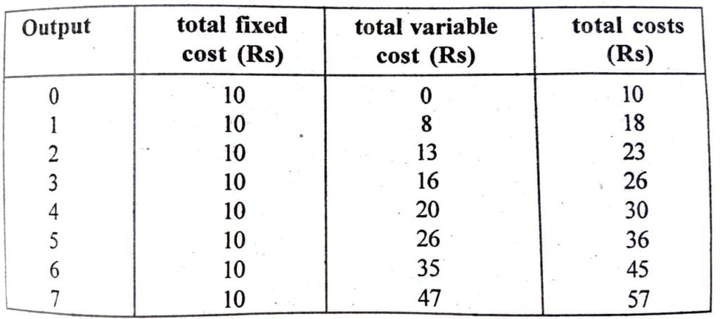
2. Show with the help of diagram that the total cost is the vertical sum of total fixed cost and total variable cost.
Ans : The total money cost incurred in producing a given quantity of production is called total cost of a firm. Total cost (TC)=Total fixed cost (TFC) + Total Variable cost (TVC)
According to Dooley, “Total cost of production is the sum of all expenditure incurred in producing a given volume of output” Total fixed costs do not change with the change in volume of output, whether the output is zero or maximum, fixed cost remain the same. In the words of Anatal Murad.
“Fixed costs are costs which do not change with change in the quantity of output.”
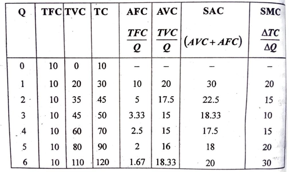
Total variable costs are those, which are incurred on the use of variable factors. Variable cost is one, which varies as the level of output varies.The relation between total fixed cost, total variable cost and total costs explained with the help of table and figure below―
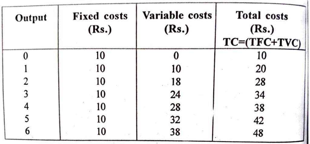
In the above table, total costs can be uneven by aggregating fixed costs and variable costs, with increase in output, total costs are also increasing. When output is zero, total costs are Rs. 10, because fixed costs are Rs. 10 although variable costs are zero, when output increase to 6 units total costs go up to Rs. 48 (38+10)
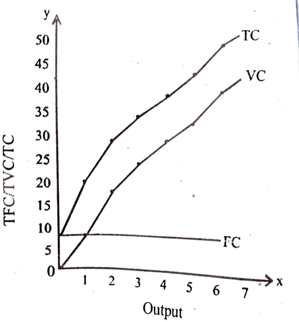
In the figure, units of output are shown on ox axis and costs on oy axis. FC line represents fixed costs, VC is variable costs curve and TC is total cost curve. TC curve begins from the starting point of curve. At point ‘O’, output is zero, but fixed cost is Rs.10, so total cost Rs. 10. Difference between total cost and variable cost is uniform and it is equivalent to fixed cost. That is why the distance between total cost curve and total variable cost curve is uniform throughout their length.
3. Show the relationship of short-run marginal cost, average variable cost and average cost with the help of curve and explain.
Ans : All aspects of short period costs like fixed cost (FC), variable cost (VC), average fixed cost (AFC), average variable cost (AVC), average cost (AC) and marginal cost (MC) are shown together in the diagram.
In the diagram, average fixed fixed cost (AFC), average variable cost (AVC) curve is continuously falling downwards, because as production increases, AFC falls. Initially, it falls sharply, later the rate of fall slows down. AVC is average variable cost. Point ‘A’ is its lowest point. After point ‘A’, this curve rises upward. AC is short period average cost (AC). As it is clear from the above diagram, the gap between average cost and average variable cost becomes narrower as the production goes on increasing. The gap is due to average fixed cost. As the average fixed cost goes on falling, the difference between average cost and average variable cost becomes narrower and narrower. Marginal cost curve is also ‘U’ shaped. This curve cuts average cost (AC) curve and average variable cost curve at their lowest points. But the reason different. It is not the law of variable proportions, but he behaviour of returns to scale.
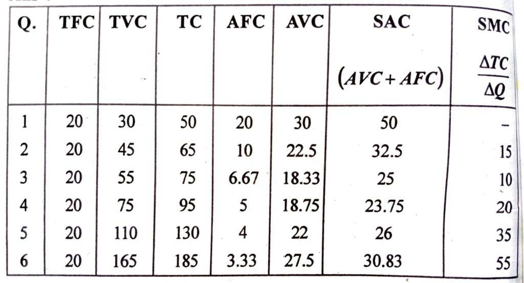
4. The short-run total cost (TC) function of a production unit is given below. Find out the total variable cost (TVC) average fixed cost (AFC), average variable cost (AVC) and average cost (AC) schedule.
Ans:
5. The production function of a production units is given as:
Q = 2L + 3K, Where K = capital and L= Labour
(i) Find out the maximum level of output, m when L=5 and K=l0.
(ii) Find out the maximum level of output, when L=6 and K=0.
Ans : Q = 5L+ 2K = 5.0+2.10 = 20 (L=0, K= 10 given)
Maximum possible output is 20 units.
6. Let the production function of a firm be given as :
Q = 5K²L², where K = capital and L=Labour.
(i) Find out the level of output when
K = 0 and L=6
(ii) Find out the level of output when
K=2 and L=3.
Solution : Q=5.(6)¹/₂0¹/₂ = 0
Q=5. (3)¹/₂. (2)¹/₂ = 5.3¹/₂. 2¹/₂=5.3¹/₂.
2¹/₂ = 5.(3.2)¹/₂+¹/₂= 5.6=30
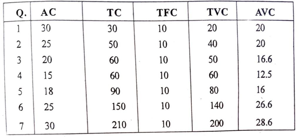
7. The short-run average cost (AC) schedule of a firm is given as below:
(i) Find out total cost (TC) schedule and marginal cost (MC)schedule.
(ii) It the total fixed cost (TFC) is Rs. 10, find out total variable cost (TVC) and average variable cost (AVC).
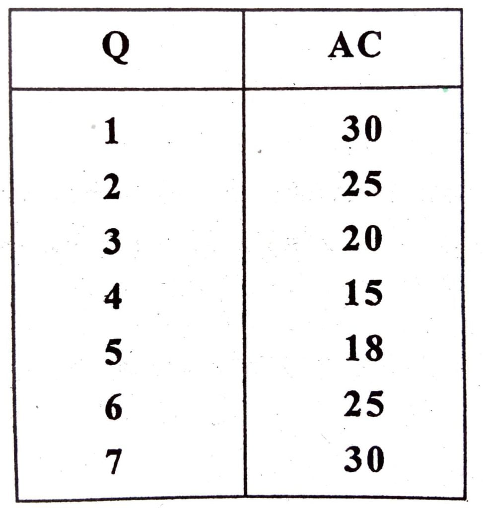
Ans:
8. The short-run total cost (TC) schedule of a firm is give below. Find out the total variable cost, total fixed cost, average cost, average variable cost and marginal cost:
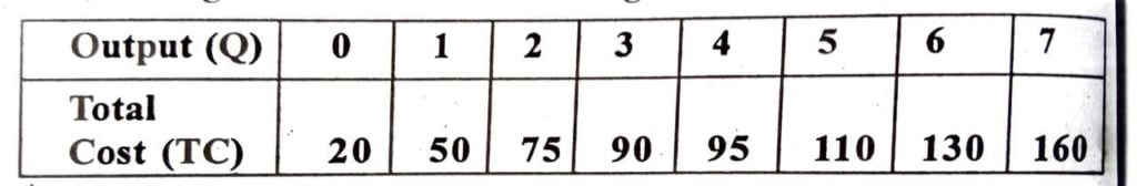
Ans:
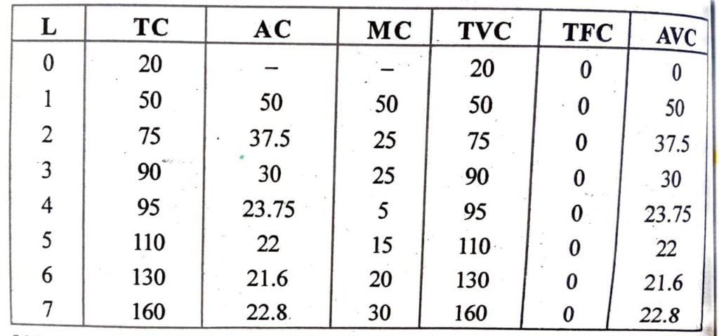
(Note: At 1st unit of output, MC= TVC=ACC, ∴ TFC=0)
9. Show different short-run cost curves and explain their natures :
Ans: Since total fixed cost remains constant at all levels of output, total fixed cost curve becomes a straight line parallel to horizontal axis.
Total variable cost curve changes with change in output. It initially increase at a decreasing rate as output increases and then it increases at increasing rate with increase in output. This is directly due to the operation of the law of variable factor. Then after a point, total variable cost starts increasing at an increasing rate. This happens because of diminishing returns to the variable factor. Three things are important regarding the behaviour of total variable cost curve. 1st, TVC is a positively sloping curve showing that as output increases. TVC also increases, second TVC curve is concave de nward in the beginning indicating that TVC increases at a decreasing rate and then beyond a output level. It is concave upward indicating that TVC increases at an increasing rate.
Third, TVC curve starts from the origin point which indicating that when output is zero. TVC is also zero. Total cost is total fixed cost plus total variable costs. Since a constant fixed cost is added to total variable cost at different levels of output the shape of TC curve is the same as that of the total variable cost curve. But total cost curve does not originate from the point of origin but from the starting point of total fixed cost. This is because total fixed cost= total cost at zero level of output. The vertical distance between the total variable cost curve and total cost curve is same at all levels of output. Therefore, like the total variable cost curve, total cost curve first increases at a decreasing rate and then at an increasing rate. This behaviour of the total cost curve directly follows from the law of Variable proportion. Three short run curve are shown in the figure below:
In the table first column shows different levels of output. In the second and third columns the values of total fixed cost and total variable cost are shown. In the fourth column total cost is shown by adding the total fixed cost and total variable cost.

Short run Average cost curve is ‘U’ shaped due to the operation of law of variable proportions dividing total cost by output we obtain the average cost. In the initial stage of production average productivity increases and therefore SAC falls. Then after a point average productivity beings to fall to causes SAC to increase.
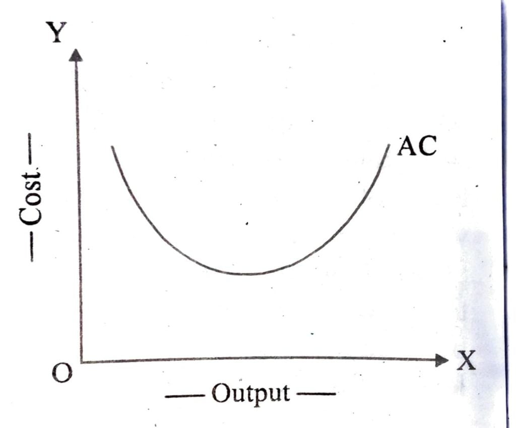
Hence, AC curve becomes ‘U’ shaped. Minium point of AC curve indicates lowest per unit cost of production.
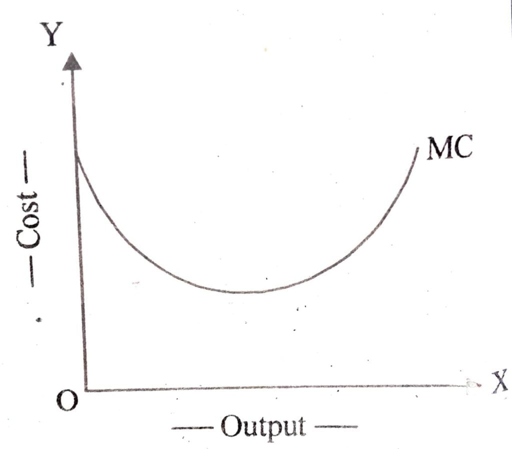
Short run marginal cost curve is also ‘U’ shaped which indicates that marginal cost falls in the beginning, then remains constant and ultimately it rises. The reason behind ‘U’ shaped of marginal cost curve is operation of law of variable proportion.
10. “Long-run marginal cost (LRMC) curve cuts the long-run average cost (LRAC)” Explain
Ans:
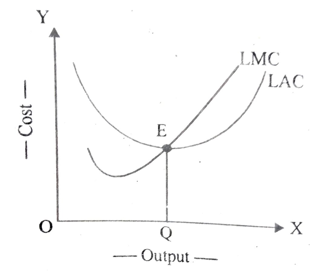
In the long run, all inputs are variable. There is no costs like fixed costs. Long run average cost curve and long run marginal cost curve are U shaped. Long run marginal cost curve cuts long run average cost curve from below at the minimum point of long run average cost curve,. It is shown in the figure below as mentioned above LAC and LMC curves are U shaped. It is because that increasing returns to scale are observed at the initial.level of production. This is then followed by the constant returns to scale and then by the diminishing returns to scale. These the ‘U’ shaped of LAC is determined by returns to scale. Its downward sloping portion corresponds to increasing returns to scale and upward portion corresponds to decreasing returns to scale. At the minimum point of LAC constant returns to scale is observed constant returns to scale may prevail over a range of output rather than at a single level of output. Hence, long run average cost will have a flat portion in the middle the figure it shows that do long as long. In run average cost is falling, LMC remains below. therefore LMC curve cuts the LAC curve at its minimum point. .
11. Explain the concept of the cost function of a typical firm with the help of an imaginary table.
Ans: Cost function means the functional relationship between cost and output. It shows total costs at each level of output. Average and marginal short run in which few inputs can be varied or for the long run in which all inputs can be varied cost function can expressed in this way C= f (Q) where C= total cost, Q= output.
A firm would always look the least cost combination of inputs for a given level of output. Therefore for a firm cost function gives the least cost combination of inputs at different level of output.
12. Distinguish between explicit cost and implicit cost. Give one example of each of them.
Ans : An implicit cost is a cost that has occurred but it is not initially shown or reported as a separate cost. On the other hand, an explicit cost is one that has occurred and is clearly reported as a separate cost. Below are some examples to illustrate the difference between an implicit cost and an explicit cost. The explicit cost of something is an actual expense that is incurred. For example, you buy a new SUV for $30,000. That’s $30,000 that you legitimately have to pay (or pay back in loans) out of pocket. Most companies and individuals think that explicit costs are the only type of costs that they incur. After all, it doesn’t cost you anything if you don’t actually see the money leaving your wallet (or bank account), right? Wrong.Implicit costs are exactly what they seem to be, implied. Think of this as an opportunity cost, or what you give up in order to do something else The general explanation is the following: your first choice for lunch isa hamburger and your second choice is pizza. What is the opportunity cos of eating a hamburger? The answer is the pizza. It’s what you have because you choose something else.
13. Find out the equilibrium quantity of output (Q).
Ans: Equilibrium quantity of output (Q) is 5 units because at this level of output MC=MR and after this output level is MC―MR.

Hi, I’m Dev Kirtonia, Founder & CEO of Dev Library. A website that provides all SCERT, NCERT 3 to 12, and BA, B.com, B.Sc, and Computer Science with Post Graduate Notes & Suggestions, Novel, eBooks, Biography, Quotes, Study Materials, and more.
